How to use Google BigQuery ML and Data Studio for exploratory data analysis

Aug. 19, 2020 | By: Pradipta Dhar

The solution? Platforms like Google BigQuery ML, which organizations can use to leverage AI by expanding their data science teams with existing business and data analysts—using only structured query language (SQL) dialects that most data teams know. BigQuery, combined with Google Data Studio, enables us to implement many different scenarios, and chief among them are data warehousing and machine learning.

In this article, you’ll learn how to analyze raw data using BigQuery and how to eventually use it to clean, shape and structure data to be used as input for machine-learning models.

What is BigQuery?

BigQuery is a cloud service offered by Google. It is primarily a data warehousing tool that can handle data at very high scales. Additionally, it can also be utilized for building machine-learning models without the knowledge of Python or R. Using BigQuery, we can build, validate and deploy machine-learning models for predicting real-world outputs.

What is exploratory data analysis?

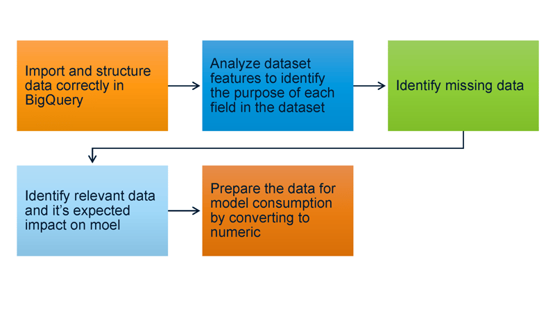
EDA refers to the process of analyzing datasets to identify their main features with the aid of visual tools. By performing EDA, we can detect missing data values, outlier points and other anomalies in the dataset. How do we perform EDA using BigQuery?

STEP 1: Select a dataset and import it into BigQuery

The dataset that we have chosen for this example is an open-source dataset from Kaggle called “Student Performance.”
Upload the CSV file containing the data into a Google Cloud Storage bucket and then import it to BigQuery. Once the dataset is imported, we can view it in the BigQuery console as shown below.

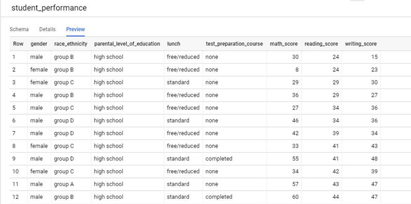
Now that we have our dataset imported into BigQuery, we are ready to start exploring and analyzing the data.

When looking at the example dataset, you’ll notice many different field representations:

• Gender: This field contains only two possible values and can be a contributing factor in scenarios where the data needs to be grouped by the gender of the student.
• Race_ethnicity: This field contains the information about what racial group the student identifies with.
• Parental_level_of_education: This field contains information about what the student’s parents’ highest educational qualification is.
• Lunch: This field tells us which lunch plan the student opts for, which could be an indicator of the student’s family’s financial situation.
• Test_preparation_course: This field tells us if the student had taken up preparatory courses before exams, and it could be a very reliable factor in determining how well the student performs in examinations.
• Math_score/Reading_score/Writing_score: These fields contain the marks obtained by the students in the respective subjects.

After understanding the different fields are and what they represent, we can dig deeper into the values contained in these fields with the help of BigQuery, as well as Google Data Studio.

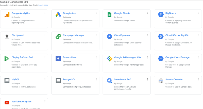
What is Google Data Studio?

Google Data Studio is Google’s cloud service for reporting and dashboard creation. It provides flexible and easy-to-use customizations that can be easily integrated with several different sources using Google Connectors, which are built-in and supported by Data Studio as shown below. Apart from the native Google Connectors, there are many Partner Connectors that have been built and support Google Data Studio connection to external data sources. Data Studio can be easily used with BigQuery for maximum analysis and visualization.

STEP 2: Discover missing values

It’s important to check for any missing values or patterns of holes in the data, which you can do with common functions. Since we have a very small dataset in the example, a quick spot check reveals that there are no fields with missing values in them.

STEP 3: Evaluate which data is relevant

Use the following query to count the total number of male versus female students, while generating a visual representation using Google Data Studio integrated with BigQuery.

select gender as GENDER, count(*) as COUNT
from student_performance
group by gender

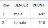
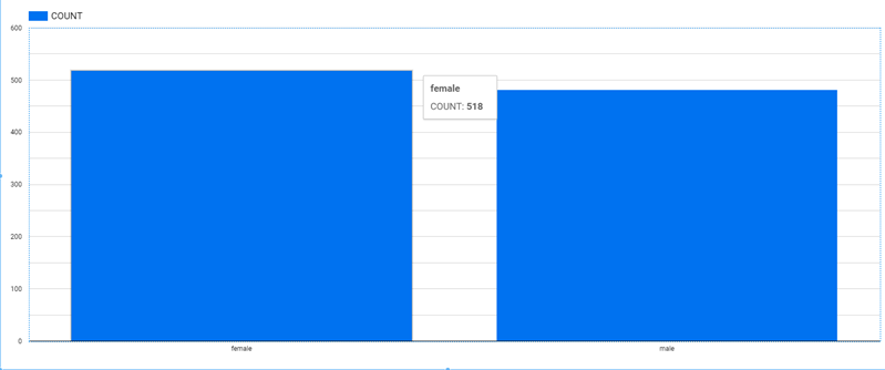
Since the dataset has almost equal distribution of male and female students, we have a decent distribution of data that can be used to train a machine-learning model with respect to the gender field, where our output label is to see if a student scores an average of above 50 in all three courses.

The next query shows us the distribution of male versus female students who have an average of more than 50.

select gender as GENDER, count(*) as Count
from student_performance
where (math_score+reading_score+writing_score)/3 >= 50
group by gender

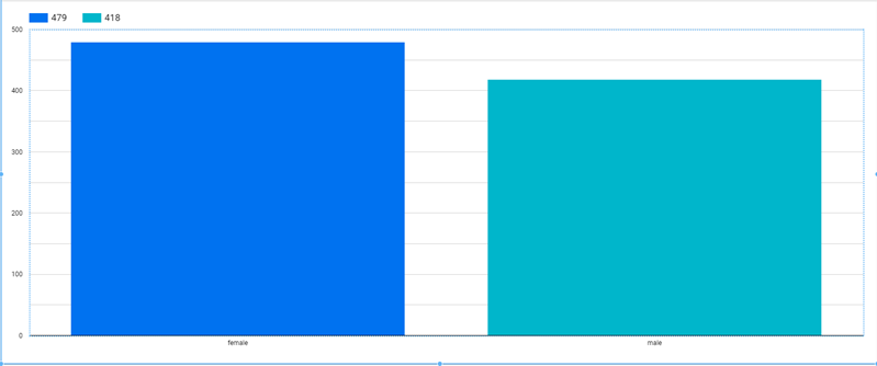
This shows us that the number of students who have an average score above 50 is proportional to the number of students belonging to each gender.

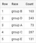
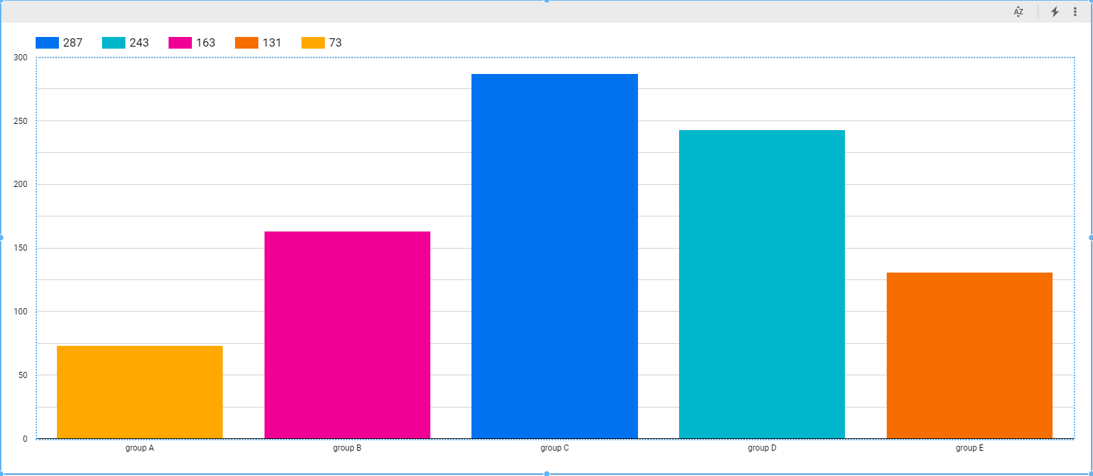
Next, observe the distribution of students that score above 50 after grouping by “race.” You’ll find that the data is well-distributed with a slightly lower count for records belonging to Race Group A, which may result in a slight skew in our training.

select race_ethnicity as Race, count(*) as Count
from student_performance
where (math_score+reading_score+writing_score)/3 >= 50
group by race_ethnicity

Next, take a look at the parental education feature:

select parental_level_of_education as Parental_Level_of_Education, count(*) as Count
from student_performance
where (math_score+reading_score+writing_score)/3 >= 50
group by parental_level_of_education

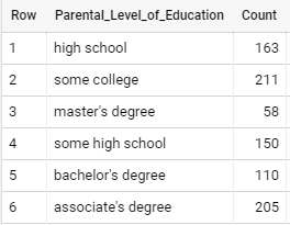
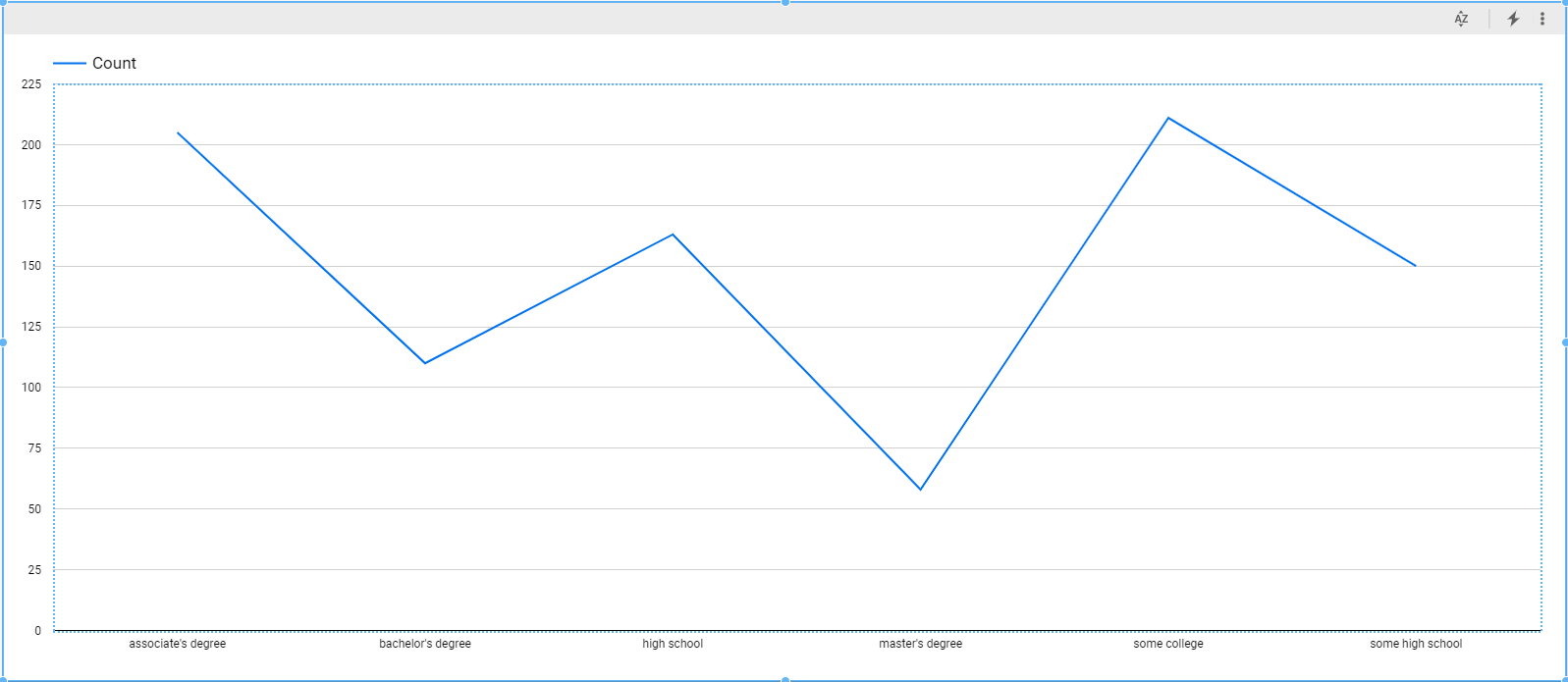
For this field again, the dataset has a slightly lower count for “Master’s Degree,” which may introduce some skew to the model.

We can analyze the remaining fields in a similar way to estimate how each field will contribute to model performance.

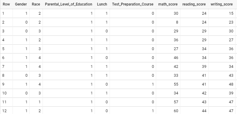
STEP 4: Prepare the data for the machine-learning model

Machine-learning models perform best when fed with numeric data instead of string data. Hence, we will convert the data in all fields into numeric representations as below:

select
  case when gender = 'male' then 1 else 0 end as Gender,
  case when race_ethnicity = 'group A' then 1 when race_ethnicity = 'group B' then 2 when    race_ethnicity = 'group C' then 3 when
race_ethnicity = 'group D' then 4 else 5 end as Race,
  case when parental_level_of_education = 'high school' then 1 when parental_level_of_education = 'some college' then 2 when parental_level_of_education = "master's degree" then 3 when parental_level_of_education = 'some high school' then 4 when parental_level_of_education = "bachelor's degree" then 5 else 6 end as
Parental_Level_of_Education,
   case when lunch = "free/reduced" then 1 else 0 end as Lunch,
   case when test_preparation_course = "completed" then 1 else 0 end as
Test_Preparation_Course,
   math_score, reading_score, writing_score
   from student_performance

Real results: Exploratory data analysis provides significant insight into data structures

By performing EDA on the dataset, organizations are able to gain valuable insight into how we can expect the various dataset features to influence model performance and how we can modify the data to be in the correct format and structure for best performance of the machine-learning model—all without even starting to build the actual machine-learning model, and without leveraging Python or R in any shape or form.

EDA’s approach to analyzing datasets is crucial to avoid rework to clean up data later, as well as any unexpected behavior of the model due to some dataset features.

Pradipta Dhar is a principal software engineer at TEKsystems with extensive expertise in machine learning and big data.